목차
- 활용 데이터셋 소개
- 환경설정 (Google Colab)
- 데이터 전처리하기
- 모델 학습 준비하기
- 모델 학습하기
- 모델 평가하기
- 소설에 모델 적용하기
- 감정 분석 결과 시각화하기
- 결과 도출하기
- 참고
한글 텍스트 자연어 처리 실습 2
1. 활용 데이터셋 소개
emotion_korTran.data
출처: Naver Cafe - nlp study: 감정분석과 감정분석 말뭉치
2. 환경설정 (Google Colab)
2.1. 환경설정 진행
# 단일 데이터셋을 다루기 위한 클래스
!pip install -q datasets
# 한글 문장 분리기
!pip install -q kss
!pip install -q pandas # 데이터 분석
!pip install -q matplotlib # 데이터 시각화
!pip install -q transformers # transformer 모델
!pip install -q gluonnlp==0.10.0
# 진행 상황 표시 모듈
!pip install -q tqdm
!pip install -q torch
!pip install -q sentencepiece
# Open Neural Network Exchange, 플랫폼 간의 모델을 교환해 사용할 수 있게 하는 모듈
!pip install -q onnxruntime
2.2. 라이브러리 import
# 모듈 임포트
import pandas as pd
import torch
from torch import nn
from torch.utils.data import Dataset, DataLoader
from transformers import BertTokenizer
from tqdm.notebook import tqdm
from transformers import AutoTokenizer, AutoModel
3. 데이터 전처리하기
3.1. 데이터 로드 및 전처리
.data -> DataFrame
data_path = "/emotion_korTran.data"

data = []
with open(data_path, "r", encoding="utf-8") as f:
    next(f)  # 첫 줄 건너뜀 (헤더)
    for line in f:
        line = line.strip()
        if not line:
            continue
        id_text = line.rsplit(",", 1)  # 오른쪽에서부터 마지막 콤마 기준으로 분할
        if len(id_text) == 2:
            idx_text, label = id_text
            idx, text = idx_text.split(",", 1)
            data.append((int(idx), text, label))

df = pd.DataFrame(data, columns=["id", "text", "label"])
전처리 된 데이터 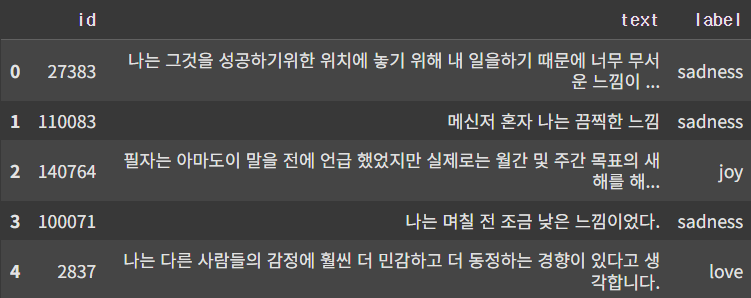
3.2. 감정 label 인코딩
label_map = {
    'joy': 0,
    'sadness': 1,
    'anger': 2,
    'fear': 3,
    'love': 4,
    'surprise': 5
}

df['label'] = df['label'].map(label_map)
4. 모델 학습 준비하기
4.1. tokenizer 및 모델 불러오기
tokenizer = AutoTokenizer.from_pretrained("monologg/kobert")
base_model = AutoModel.from_pretrained("monologg/kobert")
4.2. Dataset 클래서 정의하기
class EmotionDataset(Dataset):
    def __init__(self, texts, labels, tokenizer, max_len=64):
        self.texts = texts
        self.labels = labels # 감정 분류를 위한 감정 라벨
        self.tokenizer = tokenizer # BERT 모델 입력을 위해 토큰화 수행
        self.max_len = max_len # 입력 시퀀스를 고정 길이로 맞추기

    def __len__(self):
        return len(self.texts)

    # 모델이 학습 시 한 문장씩 꺼낼 수 있게 함
    def __getitem__(self, idx):
        encoding = self.tokenizer(
            self.texts[idx],
            padding='max_length',
            truncation=True,
            max_length=self.max_len,
            return_tensors="pt"
        )
        item = {key: val.squeeze(0) for key, val in encoding.items()}
        item["labels"] = torch.tensor(self.labels[idx])
        return item
4.3. train/validation 분할 및 DataLoader 준비하기
from sklearn.model_selection import train_test_split

# train과 validation을 9:1로 나눔
train_texts, val_texts, train_labels, val_labels = train_test_split(
    df["text"], df["label"], test_size=0.1, random_state=42
)

train_dataset = EmotionDataset(train_texts.tolist(), train_labels.tolist(), tokenizer)
# 학습 데이터 일부만 추출 (10%만) <- Colab 런타인 시간 내 학습이 완료되어야 함
data_size = len(train_dataset)
sampled_dataset = torch.utils.data.Subset(train_dataset, range(data_size//10, data_size // 10 * 2))

val_dataset = EmotionDataset(val_texts.tolist(), val_labels.tolist(), tokenizer)

train_loader = DataLoader(sampled_dataset, batch_size=32, shuffle=True)
val_loader = DataLoader(val_dataset, batch_size=32)
4.4. 분류기 모델 정의하기
# KoBERT Customizing -> PyTorch Model
class KoBERTClassifier(nn.Module):
    def __init__(self, bert, num_classes=6):
        super(KoBERTClassifier, self).__init__()
        self.bert = bert # 사전학습된 KoBERT
        self.classifier = nn.Linear(bert.config.hidden_size, num_classes) # BERT 출력 -> 감정 분류 클래스 수로 줄이는 선형 layer

    def forward(self, input_ids, attention_mask=None, token_type_ids=None):
        outputs = self.bert( # KoBERT에 입력 tensor를 넣음
            input_ids=input_ids,
            attention_mask=attention_mask,
            token_type_ids=token_type_ids
        )
        pooled = outputs.pooler_output
        return self.classifier(pooled)
5. 모델 학습하기
5.1. 모델 학습하기
colab은 12시간마다 런타임이 끊기기 때문에 학습데이터를 쪼개어서 진행했고, epoch별로 학습된 모델을 저장해줬다.
device = torch.device("cuda" if torch.cuda.is_available() else "cpu") # GPU 있으면 GPU 사용함.

model = KoBERTClassifier(base_model).to(device)
optimizer = torch.optim.AdamW(model.parameters(), lr=2e-5)
loss_fn = nn.CrossEntropyLoss()

# 저장된 모델 가중치 불러오기
model.load_state_dict(torch.load("/kobert_emotion_epoch4.pt", map_location=device))  # 파일명 확인
print("모델 가중치 불러오기 완료")

# Optimizer, Loss 재설정
optimizer = torch.optim.AdamW(model.parameters(), lr=2e-5)
loss_fn = nn.CrossEntropyLoss()

# 이어서 학습
EPOCHS = 1  # 추가로 학습할 에폭 수
start_epoch = 8  # 이어서 시작할 에폭 번호

for epoch in range(start_epoch, start_epoch + EPOCHS):
    model.train()
    total_loss = 0

    for batch in tqdm(train_loader):
        input_ids = batch['input_ids'].to(device)
        attention_mask = batch['attention_mask'].to(device)
        token_type_ids = batch['token_type_ids'].to(device)
        labels = batch['labels'].to(device)

        optimizer.zero_grad()
        outputs = model(input_ids, attention_mask, token_type_ids)
        loss = loss_fn(outputs, labels)
        loss.backward()
        optimizer.step()
        total_loss += loss.item()

    avg_loss = total_loss / len(train_loader)
    print(f"[Epoch {epoch}] Loss: {avg_loss:.4f}")
5.2. 모델 저장하기
from google.colab import files

# 에폭별 모델 저장
model_path = f"/kobert_emotion_epoch{epoch+1}.pt"
drive_path = f"/{model_path}"

# 로컬에 저장
torch.save(model.state_dict(), model_path)

# model 다운로드
files.download(model_path)
7. 모델 평가하기
device = torch.device("cuda" if torch.cuda.is_available() else "cpu")

# 모델 구조 다시 정의 (기존과 동일하게)
model = KoBERTClassifier(base_model).to(device)

# 저장된 가중치 불러오기
model_path = "/content/drive/MyDrive/Colab Notebooks/NLP/models/kobert_emotion_epoch8.pt"
model.load_state_dict(torch.load(model_path, map_location=device))

# 평가 모드로 전환
model.eval()
from sklearn.metrics import accuracy_score

def evaluate_accuracy(model, dataloader, tokenizer, sample_texts=None):
    model.eval()
    preds = []
    true_labels = []
    sample_outputs = []

    with torch.no_grad():
        for batch in tqdm(dataloader):
            input_ids = batch['input_ids'].to(device)
            attention_mask = batch['attention_mask'].to(device)
            token_type_ids = batch['token_type_ids'].to(device)
            labels = batch['labels'].to(device)

            outputs = model(input_ids, attention_mask, token_type_ids)
            predictions = torch.argmax(outputs, dim=1)

            preds.extend(predictions.cpu().numpy())
            true_labels.extend(labels.cpu().numpy())

            # 샘플 출력용 텍스트 복원
            if sample_texts and len(sample_outputs) < 10:
                texts = sample_texts[len(sample_outputs):len(sample_outputs)+len(predictions)]
                for text, pred, true in zip(texts, predictions, labels):
                    sample_outputs.append((text, pred.item(), true.item()))
                    if len(sample_outputs) == 10:
                        break

    acc = accuracy_score(true_labels, preds)
    print(f"Validation Accuracy: {acc * 100:.2f}%\n")
evaluate_accuracy(model, val_loader, tokenizer)

8. 해리포터 소설에 감정 분석 모델 적용하기
# 해리포터 소설 불러오기
with open("해리포터_통합본_전처리.txt", "r", encoding="utf-8") as f:
    texts = f.read().split('\n')

# 해리포터 전권을 챕터별로 구분
chapters = []
chapter_titles = []
chapter = []
chapter_length = []
cnt = 0

chapter_titles.append(texts[0])
for i in range(1, len(texts)):
    if texts[i].strip():
        if re.match(r'제\s*\d+\s*장\s*[^\n]*\n?', texts[i]):
            chapter_titles.append(texts[i])
            chapters.append(chapter)
            chapter = []
            chapter_length.append(cnt)
            cnt = 0
        else:
            chapter.append(texts[i])
            cnt += 1
def predict_emotion(sentence, model, tokenizer):
    model.eval() # 평가 모드로 변경

    encoding = tokenizer(
        sentence,
        return_tensors='pt',
        padding='max_length',
        truncation=True,
        max_length=64
    )

    input_ids = encoding['input_ids'].to(device)
    attention_mask = encoding['attention_mask'].to(device)
    token_type_ids = encoding.get('token_type_ids', torch.zeros_like(input_ids)).to(device)

    with torch.no_grad():
        output = model(input_ids, attention_mask, token_type_ids)
        prediction = torch.argmax(output, dim=1).item()

    label_map_reverse = {
        0: '기쁨', 1: '슬픔', 2: '분노', 3: '불안', 4: '사랑', 5: '놀람'
    }

    return label_map_reverse[prediction]
import pandas as pd
from tqdm import tqdm

for i, chapter in enumerate(zip(chapter_titles, chapters)):
    title = chapter[0]
    sentences = chapter[1]
    results = []

    for sentence in tqdm(sentences, desc=f"'{title}' 감정 분석 중"):
        emotion = predict_emotion(sentence, model, tokenizer)
        results.append({
            "sentence": sentence,
            "emotion": emotion
        })

    # DataFrame으로 변환
    df = pd.DataFrame(results)

    # CSV 파일로 저장
    filename = f"{title}.csv"
    df.to_csv(filename, index=False, encoding='utf-8-sig')  # 윈도우 한글 호환
    print(f"저장 완료: {filename}")
9. 감정 분석 결과 시각화
# 사용할 감정 라벨
emotion_labels = ['기쁨', '슬픔', '분노', '불안', '놀람', '사랑']

# 각 감정의 극성 점수 (valence)
emotion_score = {
    '기쁨': 3, '사랑': 2, '놀람': 1,
    '불안': -1, '슬픔': -2, '분노': -3
}
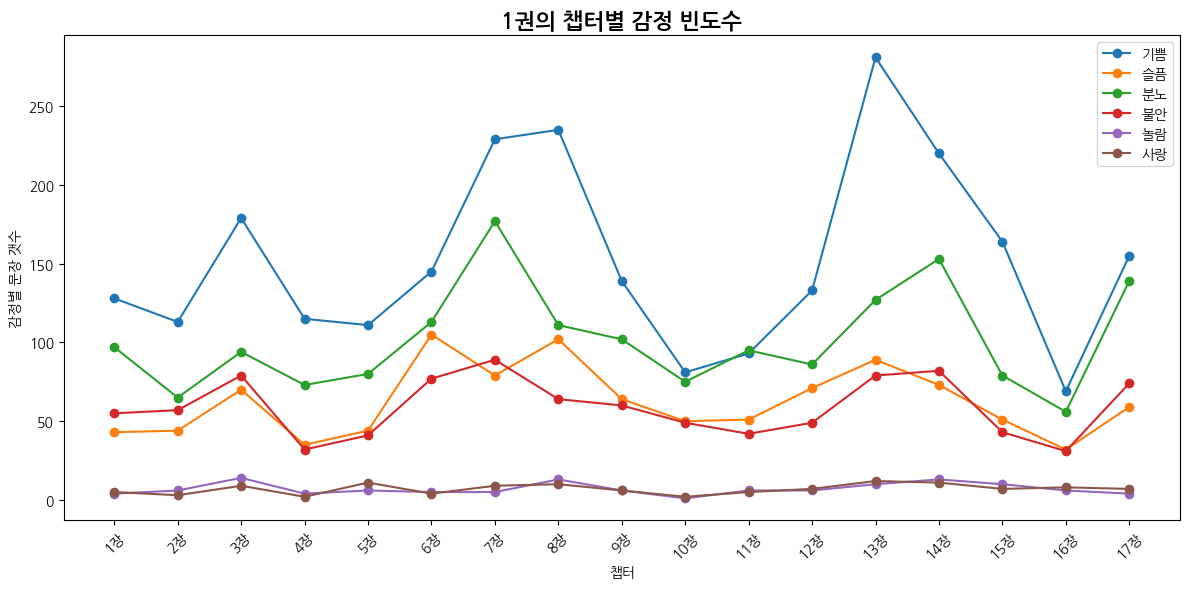
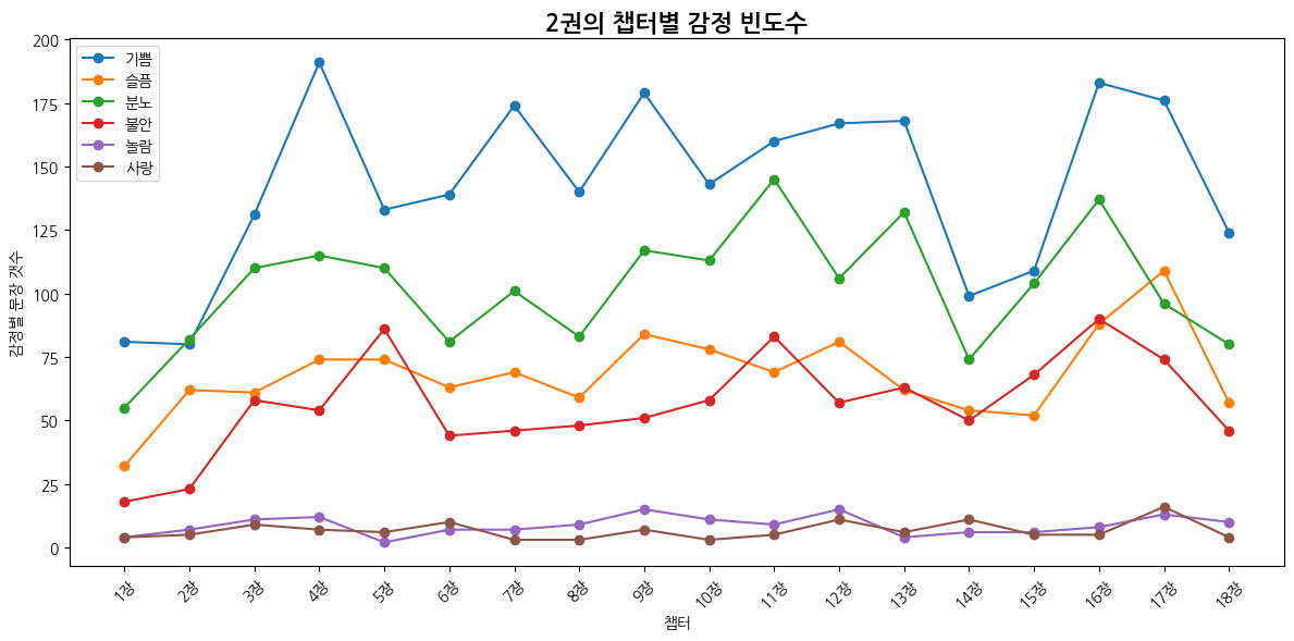
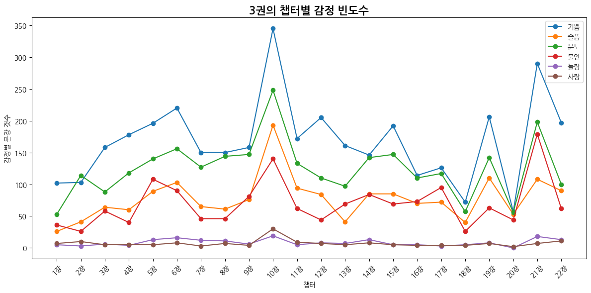
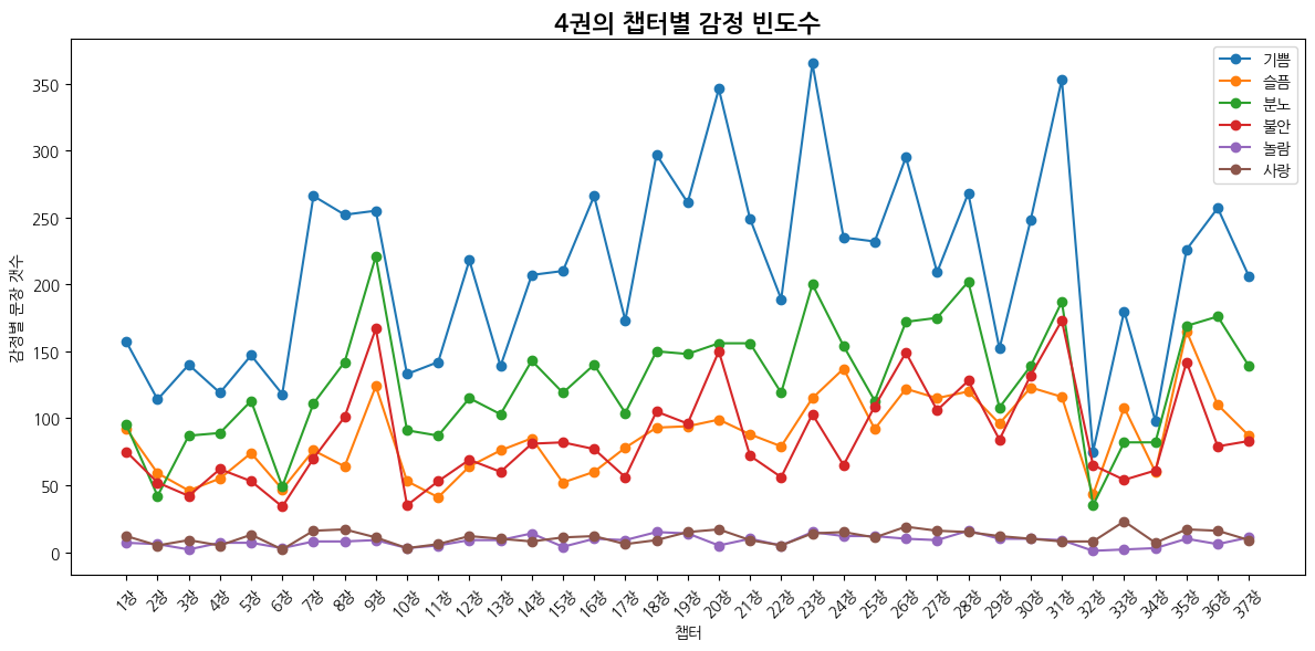
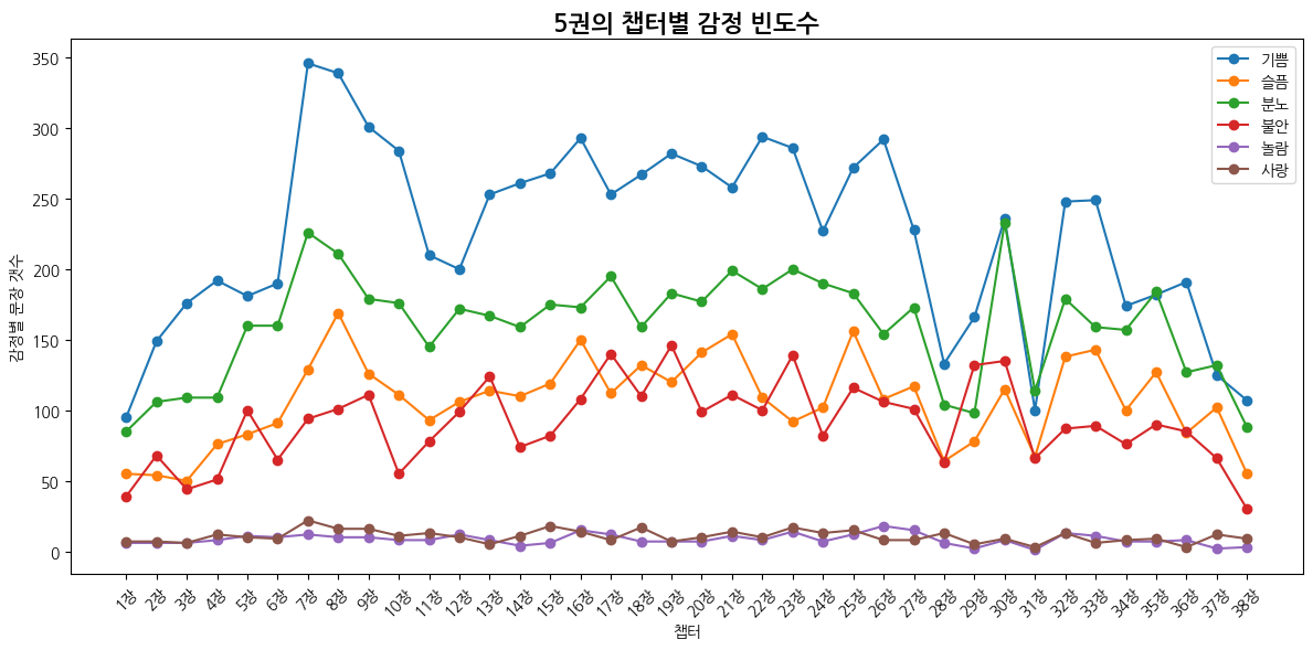
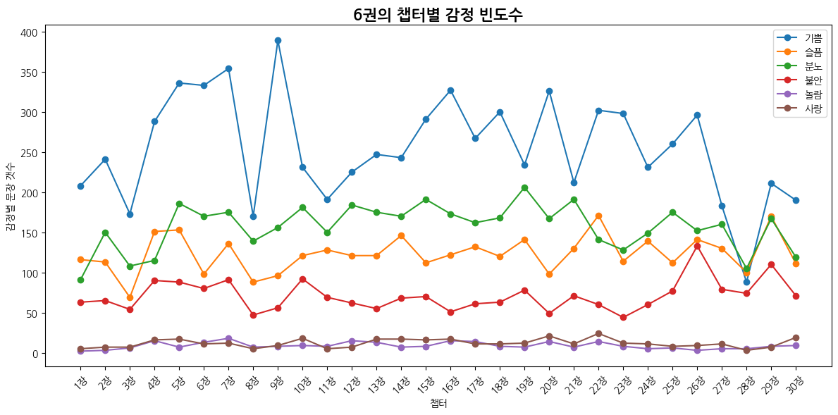
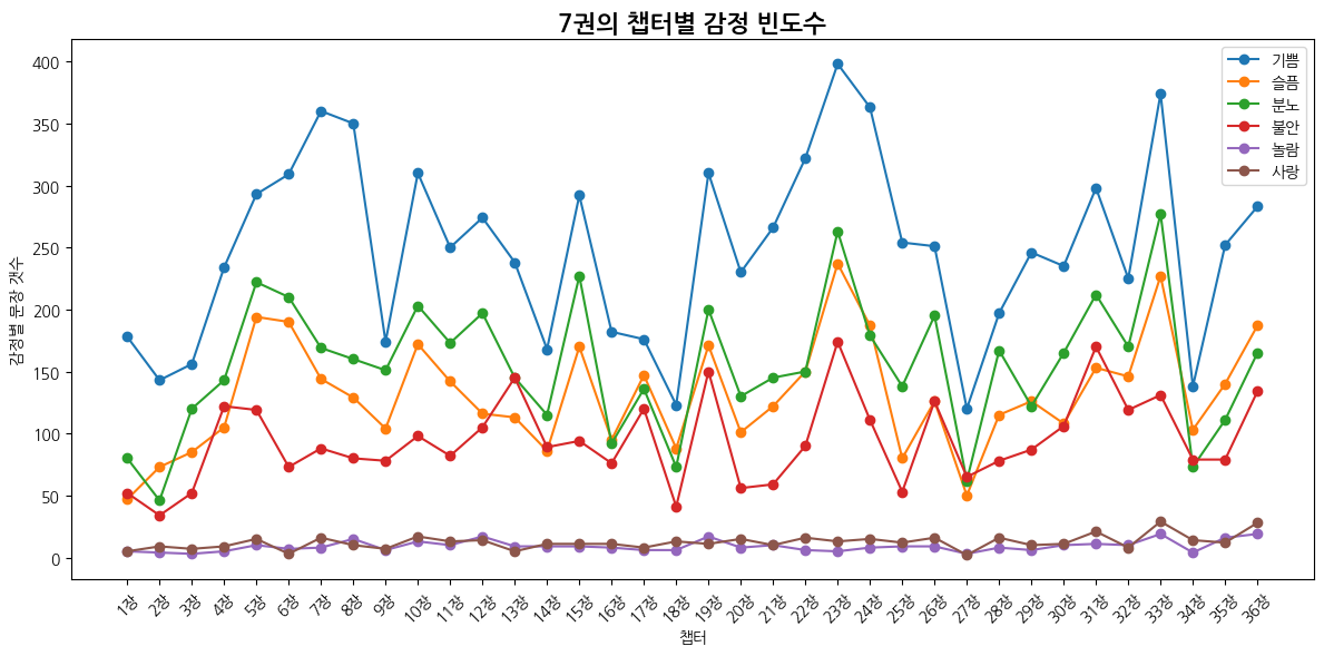
def emotion_frequency_flow(emotion_df):
    # 감정 흐름 시각화
    plt.figure(figsize=(12, 6))

    for label in emotion_labels:
        x = [f'{i+1}장' for i in range(len(emotion_df))]
        y = emotion_df[label]
        plt.plot(x, y, marker='o', label=label)

    plt.title("챕터별 감정 빈도수")
    plt.xlabel("챕터")
    plt.ylabel("감정별 문장 갯수")
    plt.xticks(rotation=45)

    plt.legend()
    plt.tight_layout()
    plt.show()
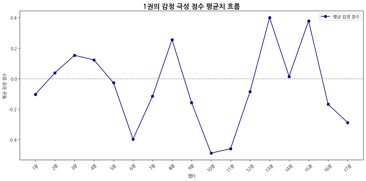
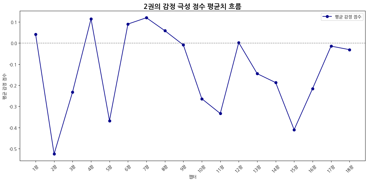
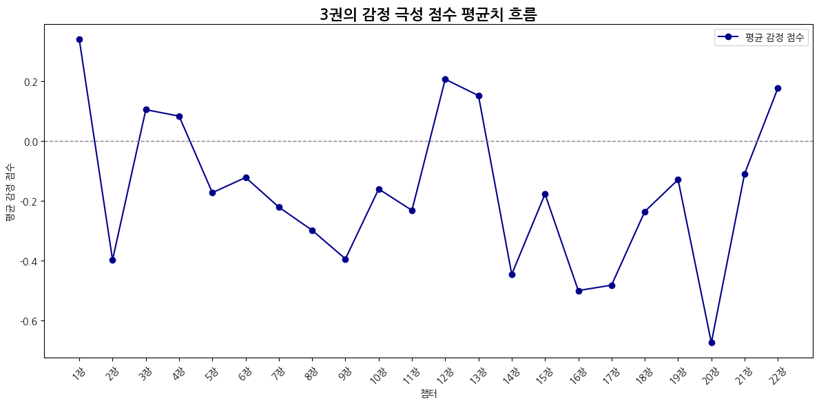
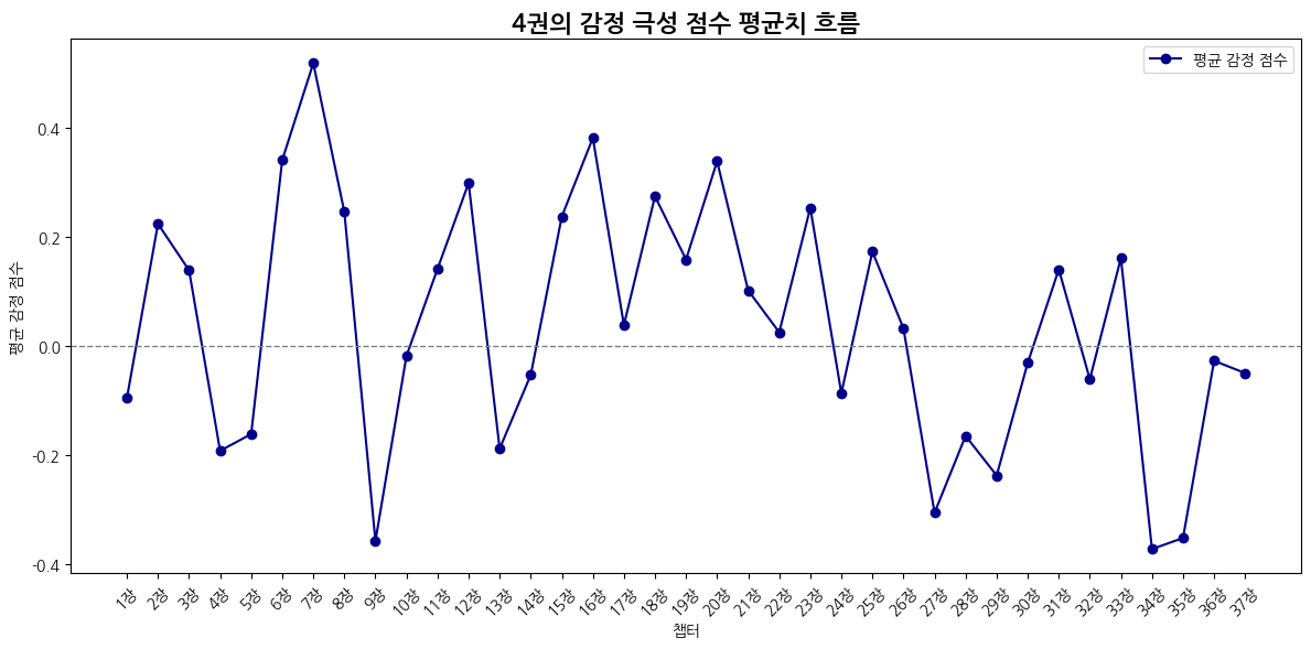
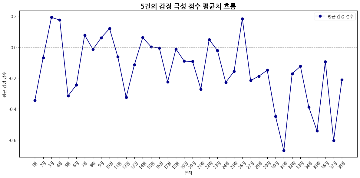
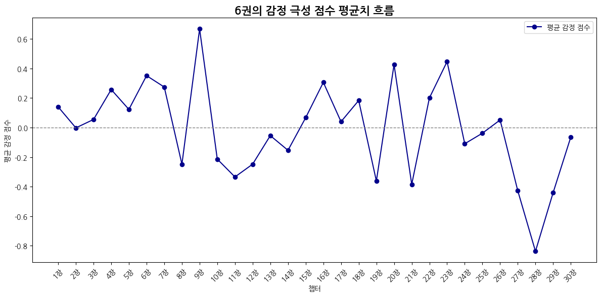
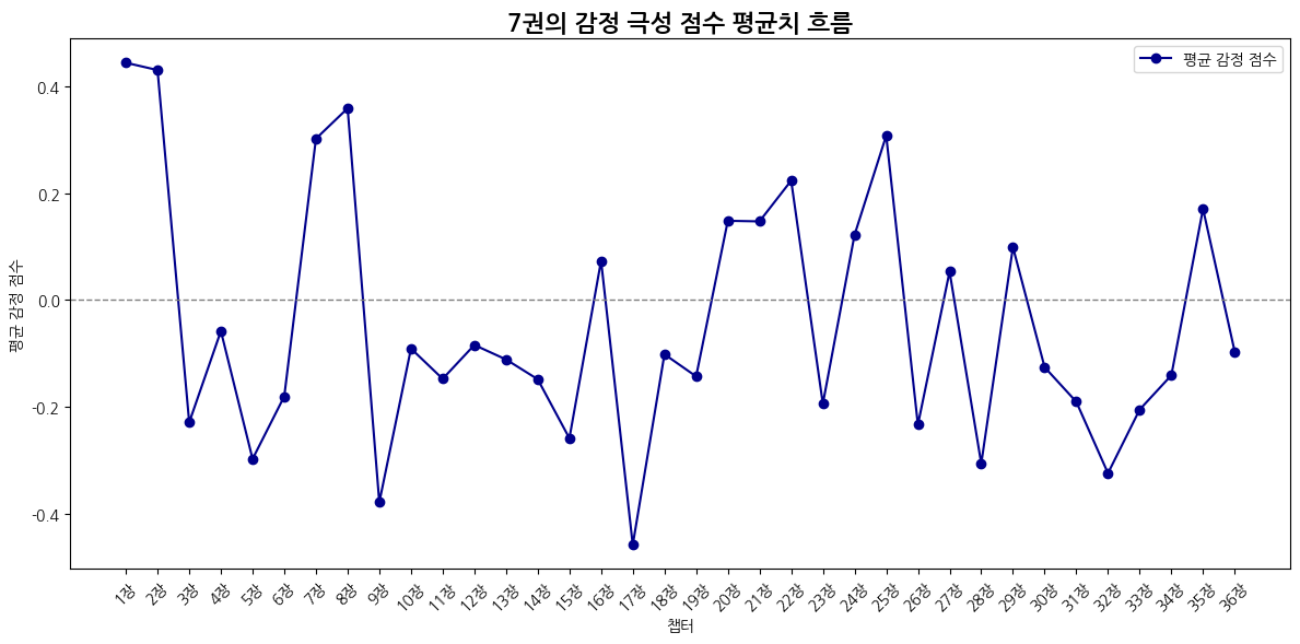
평균값은 (감정 극성값 * 빈도수)의 합 / 전체 문장 수
# 감정 극성 평균값을 기반으로 흐름만 시각화
def emotion_avg_score_flow(emotion_df):
    plt.figure(figsize=(12, 6))

    x = [f'{i+1}장' for i in range(len(emotion_df))]
    y = emotion_df['avg_emotion_score']

    plt.plot(x, y, marker='o', color='darkblue', label='평균 감정 점수')

    plt.title("감정 극성 점수의 평균치 흐름")
    plt.xlabel("챕터")
    plt.ylabel("평균 감정 점수")
    plt.axhline(0, color='gray', linestyle='--', linewidth=1)
    plt.xticks(rotation=45)

    plt.legend()
    plt.tight_layout()
    plt.show()
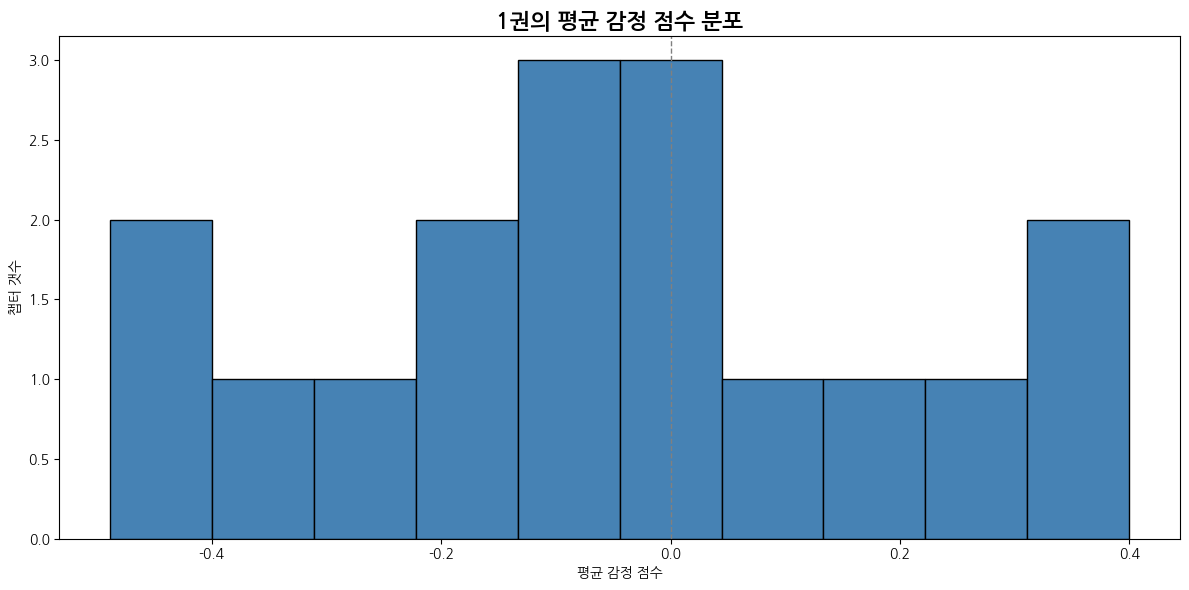
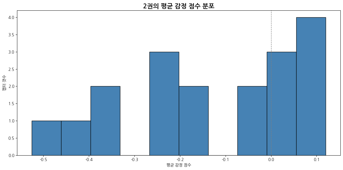
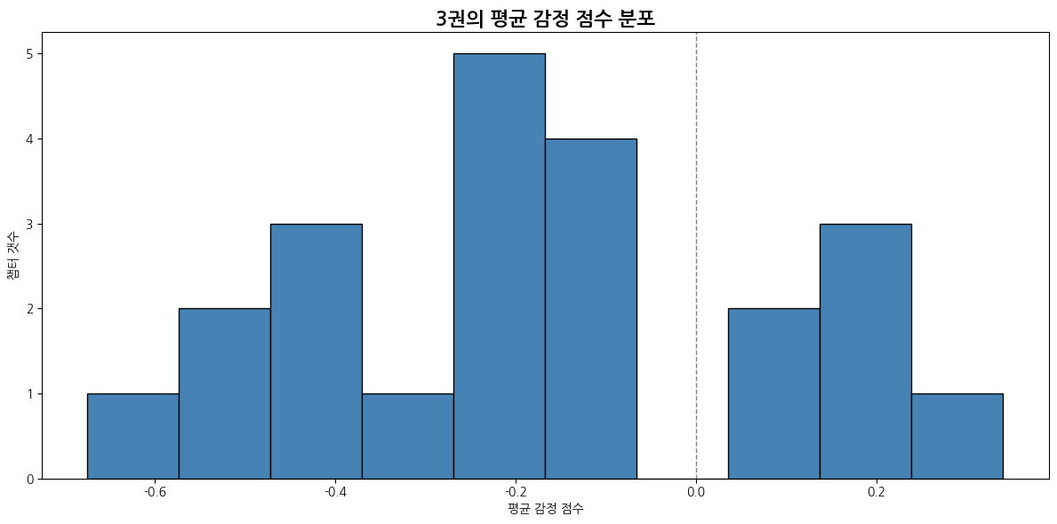
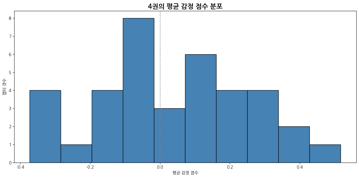
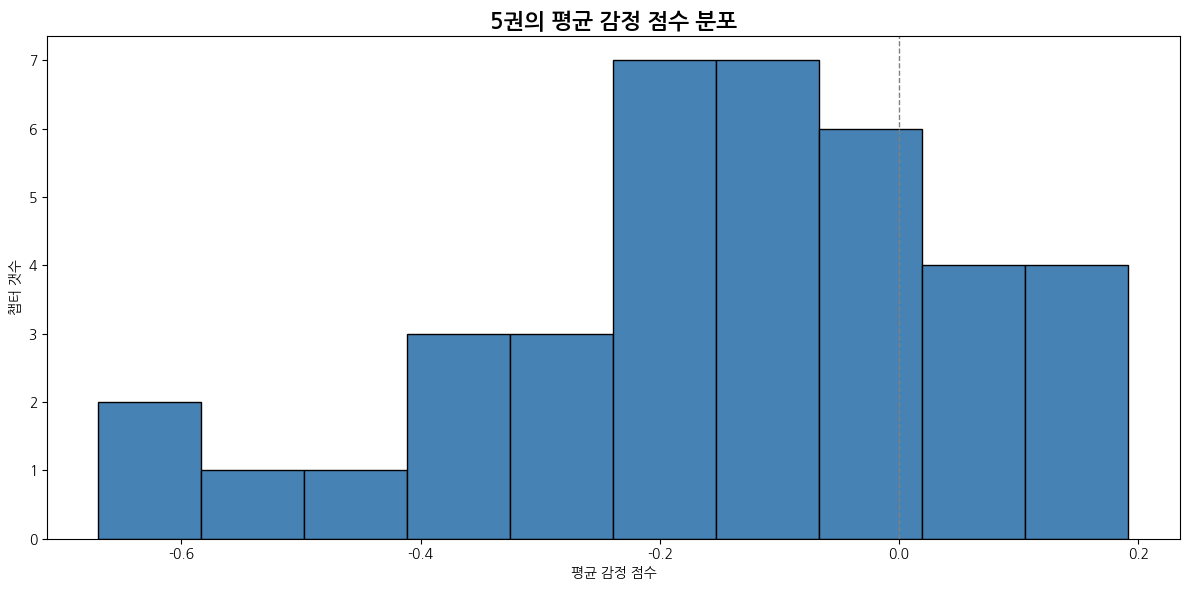
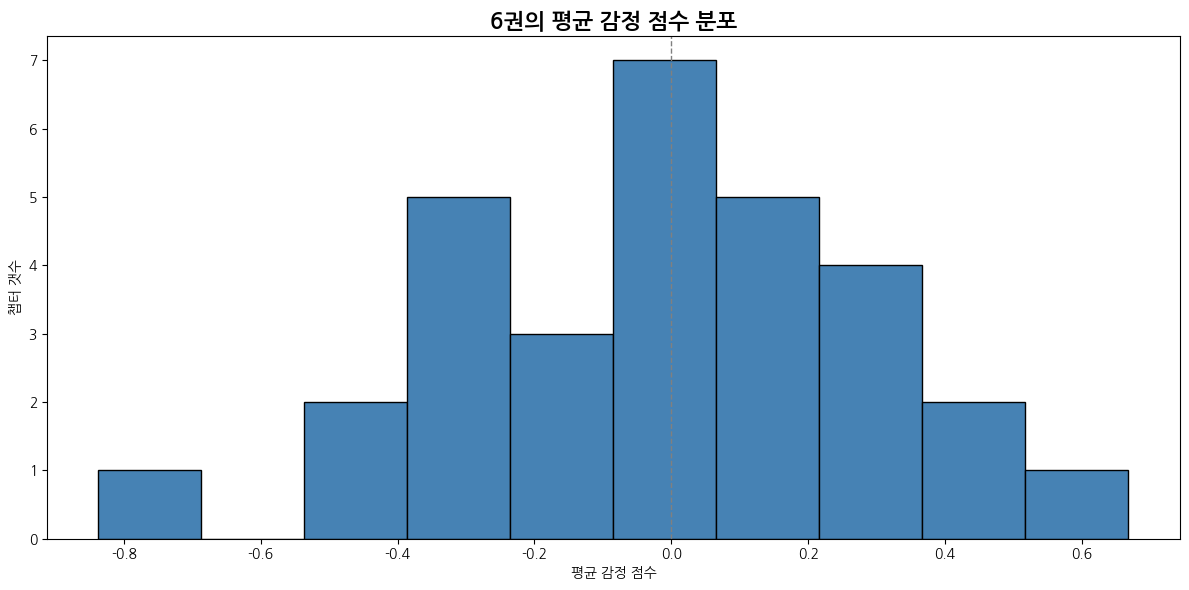
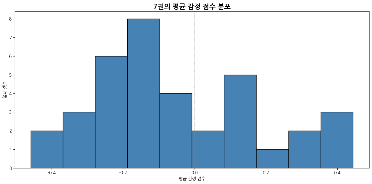
# 평균 감정 점수의 분포를 히스토그램으로 시각화
def emotion_score_histogram(emotion_df):
    plt.figure(figsize=(12, 6))

    plt.hist(emotion_df['avg_emotion_score'], bins=10, color='steelblue', edgecolor='black')

    plt.title("평균 감정 점수 분포")
    plt.xlabel("평균 감정 점수")
    plt.ylabel("챕터 갯수")
    plt.axvline(0, color='gray', linestyle='--', linewidth=1)

    plt.tight_layout()
    plt.show()
# 감정별로 가장 우세한 챕터 상위 3개를 dictionary 형태로 반환

def get_chapter_dominance_by_emotion_dict(emotion_df, top_n=3):
    emotion_labels = ['기쁨', '슬픔', '분노', '불안', '놀람', '사랑']
    emotion_totals = {emotion: emotion_df[emotion].sum() for emotion in emotion_labels}

    dominance_dict = {}

    for emotion in emotion_labels:
        dominance_rows = []
        for _, row in emotion_df.iterrows():
            chapter = row['chapter']
            value = row[emotion]
            dominance_ratio = value / emotion_totals[emotion] if emotion_totals[emotion] > 0 else 0
            dominance_rows.append((chapter, round(dominance_ratio, 3)))

        top_chapters = sorted(dominance_rows, key=lambda x: x[1], reverse=True)[:top_n]
        dominance_dict[emotion] = top_chapters

    return dominance_dict
def analyze_emotion_structure(folder_path):
    chapter_emotions = []

    # 각 챕터 파일에서 감정 통계 집계
    for filename in sorted(os.listdir(folder_path)):
        if filename.endswith(".csv"):
            filepath = os.path.join(folder_path, filename)
            df = pd.read_csv(filepath)
            chapter_name = filename.replace(".csv", "")

            # 감정 빈도 수 계산
            emotion_counts = df['emotion'].value_counts().to_dict()
            row = {'chapter': chapter_name}
            total = 0
            score_sum = 0

            for label in emotion_labels:
                count = emotion_counts.get(label, 0)
                row[label] = count
                total += count
                score_sum += emotion_score.get(label, 0) * count

            row['total'] = total
            row['avg_emotion_score'] = score_sum / total if total > 0 else 0
            chapter_emotions.append(row)

    # 데이터프레임 생성
    emotion_df = pd.DataFrame(chapter_emotions)
    emotion_df = emotion_df.sort_values('chapter').reset_index(drop=True)
    emotion_df.fillna(0, inplace=True)

    # 그래프 시각화
    emotion_avg_score_flow(emotion_df)
    emotion_frequency_flow(emotion_df)
    emotion_score_histogram(emotion_df)

    # 특정 감정 많은 챕터 추출
    top_chapters_by_emotion = get_chapter_dominance_by_emotion_dict(emotion_df)

    return emotion_df, top_chapters_by_emotion
for (path, dirs, files) in os.walk(root_path):
    for dir in sorted(dirs):
        folder_path = path + '/' + dir  # 각 챕터 감정 CSV 폴더 경로
        emotion_df, top_chapters_by_emotion = analyze_emotion_structure(folder_path)
        # 감정 구조 분석 결과
        print(emotion_df.head())
        for label in emotion_labels:
            print(f"{label} 감정이 집중된 챕터 Top 3:")
            for k, v in top_chapters_by_emotion[label]:
                print(f"{k} 챕터: {v}")
            print()
    break
10. 결과
1권
| 감정 | 1위 챕터 | 비율 | 2위 챕터 | 비율 | 3위 챕터 | 비율 |
|---|---|---|---|---|---|---|
| 기쁨 | 5장 다이애건 앨리 | 0.108 | 17장 두 얼굴을 가진 사람 | 0.091 | 16장 지하실 문을 지나서 | 0.088 |
| 슬픔 | 15장 금지된 숲 | 0.099 | 17장 두 얼굴을 가진 사람 | 0.096 | 5장 다이애건 앨리 | 0.084 |
| 분노 | 16장 지하실 문을 지나서 | 0.103 | 6장 9와 3/4번 승강장 | 0.089 | 9장 한밤의 결투 | 0.081 |
| 불안 | 16장 지하실 문을 지나서 | 0.089 | 6장 9와 3/4번 승강장 | 0.082 | 12장 소망의 거울 | 0.079 |
| 놀람 | 12장 소망의 거울 | 0.118 | 17장 두 얼굴을 가진 사람 | 0.109 | 6장 9와 3/4번 승강장 | 0.109 |
| 사랑 | 5장 다이애건 앨리 | 0.102 | 14장 노르웨이 리지백 노버트 | 0.093 | 6장 9와 3/4번 승강장 | 0.093 |
2권
| 감정 | 1위 챕터 | 비율 | 2위 챕터 | 비율 | 3위 챕터 | 비율 |
|---|---|---|---|---|---|---|
| 기쁨 | 4장 플러리시와 블러트 서점에서 | 0.074 | 16장 비밀의 방 | 0.071 | 9장 벽면에 쓰여진 경고 | 0.069 |
| 슬픔 | 17장 슬리데린의 후계자 | 0.089 | 16장 비밀의 방 | 0.072 | 9장 벽면에 쓰여진 경고 | 0.068 |
| 분노 | 11장 결투클럽 | 0.079 | 16장 비밀의 방 | 0.074 | 13장 비밀 일기 | 0.072 |
| 불안 | 16장 비밀의 방 | 0.088 | 5장 커다란 버드나무 | 0.085 | 11장 결투클럽 | 0.082 |
| 놀람 | 9장 벽면에 쓰여진 경고 | 0.096 | 12장 폴리주스 마법의 약 | 0.096 | 17장 슬리데린의 후계자 | 0.083 |
| 사랑 | 17장 슬리데린의 후계자 | 0.133 | 12장 폴리주스 마법의 약 | 0.092 | 14장 코넬리우스 퍼지 | 0.092 |
3권
| 감정 | 1위 챕터 | 비율 | 2위 챕터 | 비율 | 3위 챕터 | 비율 |
|---|---|---|---|---|---|---|
| 기쁨 | 10장 호그와트의 비밀지도 | 0.093 | 21장 헤르미온느의 비밀 | 0.078 | 6장 갈고리 발톱과 찻잎 | 0.059 |
| 슬픔 | 10장 호그와트의 비밀지도 | 0.113 | 19장 볼트모트의 부하 | 0.064 | 21장 헤르미온느의 비밀 | 0.063 |
| 분노 | 10장 호그와트의 비밀지도 | 0.090 | 21장 헤르미온느의 비밀 | 0.072 | 6장 갈고리 발톱과 찻잎 | 0.057 |
| 불안 | 21장 헤르미온느의 비밀 | 0.116 | 10장 호그와트의 비밀지도 | 0.091 | 5장 디멘터 | 0.070 |
| 놀람 | 10장 호그와트의 비밀지도 | 0.103 | 21장 헤르미온느의 비밀 | 0.097 | 6장 갈고리 발톱과 찻잎 | 0.086 |
| 사랑 | 10장 호그와트의 비밀지도 | 0.191 | 22장 다시 온 부엉이 집배원 | 0.070 | 2장 마지막 아주머니의 큰 실수 | 0.064 |
4권
| 감정 | 1위 챕터 | 비율 | 2위 챕터 | 비율 | 3위 챕터 | 비율 |
|---|---|---|---|---|---|---|
| 기쁨 | 23장 크리스마스 무도회 | 0.047 | 31장 세 번째 시험 | 0.045 | 20장 첫번째 시험 | 0.044 |
| 슬픔 | 35장 베리타세룸 | 0.051 | 24장 리타 스키터의 특종 기사 | 0.043 | 9장 어둠의 표시 | 0.039 |
| 분노 | 9장 어둠의 표시 | 0.047 | 28장 크라우치의 광기 | 0.043 | 23장 크리스마스 무도회 | 0.042 |
| 불안 | 31장 세 번째 시험 | 0.054 | 9장 어둠의 표시 | 0.052 | 20장 첫번째 시험 | 0.047 |
| 놀람 | 28장 크라우치의 광기 | 0.052 | 18장 마법 지팡이 검사 | 0.049 | 23장 크리스마스 무도회 | 0.049 |
| 사랑 | 33장 죽음을 먹는 자들 | 0.056 | 26장 두 번째 시험 | 0.046 | 8장 퀴디치 월드컵 | 0.041 |
5권
| 감정 | 1위 챕터 | 비율 | 2위 챕터 | 비율 | 3위 챕터 | 비율 |
|---|---|---|---|---|---|---|
| 기쁨 | 12장 엄브릿지 교수 | 0.040 | 13장 돌로레스의 나머지 공부 | 0.040 | 14장 퍼시와 패드 풋 | 0.035 |
| 슬픔 | 13장 돌로레스의 나머지 공부 | 0.042 | 26장 본 것과 보지 못한 것 | 0.038 | 30장 그롭 | 0.038 |
| 분노 | 35장 베일 속으로 | 0.038 | 12장 엄브릿지 교수 | 0.037 | 13장 돌로레스의 나머지 공부 | 0.035 |
| 불안 | 24장 오클러먼시 | 0.042 | 22장 마법 질병과 상해를 위한 성 뭉고 병원 | 0.040 | 28장 스네이프의 가장 끔찍한 기억 | 0.040 |
| 놀람 | 31장 O.W.L.시험 | 0.055 | 21장 뱀의 눈 | 0.046 | 32장 벽난로에서 붙잡히다 | 0.046 |
| 사랑 | 12장 엄브릿지 교수 | 0.054 | 20장 해그리드의 이야기 | 0.045 | 23장 격리 병동에서의 크리스마스 | 0.042 |
6권
| 감정 | 1위 챕터 | 비율 | 2위 챕터 | 비율 | 3위 챕터 | 비율 |
|---|---|---|---|---|---|---|
| 기쁨 | 9장 혼혈 왕자 | 0.051 | 7장 민달팽이 클럽 | 0.046 | 5장 플렘의 지나친 행동 | 0.044 |
| 슬픔 | 22장 장례식이 끝난 후 | 0.046 | 29장 불사조의 슬픈 노래 | 0.046 | 4장 호레이스 슬레그혼 | 0.041 |
| 분노 | 19장 집요정의 미행 | 0.044 | 15장 깨뜨릴 수 없는 맹세 | 0.041 | 21장 알 수 없는 방 | 0.041 |
| 불안 | 26장 동굴 | 0.062 | 29장 불사조의 슬픈 노래 | 0.052 | 7장 민달팽이 클럽 | 0.043 |
| 놀람 | 7장 민달팽이 클럽 | 0.067 | 4장 호레이스 슬레그혼 | 0.056 | 12장 은잔과 오팔 목걸이 | 0.056 |
| 사랑 | 22장 장례식이 끝난 후 | 0.067 | 20장 볼드모트 경의 요구 | 0.059 | 30장 하얀 무덤 | 0.053 |
7권
| 감정 | 1위 챕터 | 비율 | 2위 챕터 | 비율 | 3위 챕터 | 비율 |
|---|---|---|---|---|---|---|
| 기쁨 | 23장 말포이 저택 | 0.044 | 33장 왕자 이야기 | 0.042 | 7장 알버스 덤블도어의 유언 | 0.040 |
| 슬픔 | 23장 말포이 저택 | 0.050 | 33장 왕자 이야기 | 0.048 | 5장 쓰러진 전사 | 0.041 |
| 분노 | 33장 왕자 이야기 | 0.050 | 23장 말포이 저택 | 0.047 | 15장 도깨비의 복수 | 0.041 |
| 불안 | 23장 말포이 저택 | 0.051 | 31장 호그와트의 전투 | 0.050 | 19장 은빛 암사슴 | 0.044 |
| 놀람 | 33장 왕자 이야기 | 0.058 | 36장 구멍 난 계획 | 0.058 | 12장 마법은 힘이다. | 0.052 |
| 사랑 | 33장 왕자 이야기 | 0.065 | 36장 구멍 난 계획 | 0.063 | 31장 호그와트의 전투 | 0.047 |
참고
- Dataset.map
- [RN] ONNX(Open Neural Network Exchange) 이해하기 -1: React Native 활용
- 전이학습(Transfer learning)과 파인튜닝(Fine tuning)
- [Python, KoBERT] 다중 감정 분류 모델 구현하기 (huggingface로 이전 방법 O)
- [KoBERT] SKTBrain의 KoBERT 공부하기
- 1.허깅페이스란?
- Hugging Face: KoBERT
- [인지과학] 사람의 감정을 어떻게 정의할 수 있을까?
- [Python] 히트맵 그리기 (Heatmap by python matplotlib, seaborn, pandas)